Technical basics series: Bayesian inference 101

Bayesian inference is a paradigm for doing statistical inference. It all comes down to Bayes’s theorem:

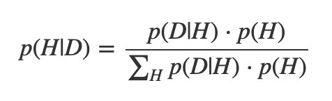
The left side is a conditional probability, and you read it as “The probability of hypothesis H being true, given that your data set is D." This probability is called the posterior probability.

Focus on the numerator. The left term is called the likelihood function. Notice that you read it as “the probability of getting data set D, given a particular hypothesis H.” In other words, the likelihood is a data-generating model for an inquiry that we have.

The right term doesn’t involve the data set at all, and expresses what we know about our hypotheses before we do any inference at all. As a result, it’s called the prior probability.

These are probabilities, and as such must be between 0 and 1. The denominator, sometimes called the evidence, is the normalizing factor.

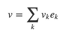
There’s a neat parallel between vectors and bases on one side and the evidence on the other. You know how you can write a vector as a weighted sum of basis vectors?

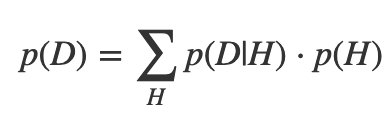
If your set of hypotheses is mutually exclusive and exhaustive, you can do a similar thing with probabilities, called The Law of Total Probability:

So Bayes’s theorem can be written more compactly:

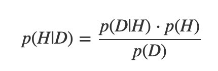
Or even:

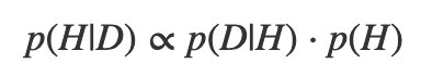
(That’s a “proportionality” symbol.) The posterior is proportional to the product of the likelihood and the prior.

All statisticians use Bayes’s theorem, even frequentists. What makes you a Bayesian is in how you interpret it. A Bayesian can treat “H” and “D” as degrees of belief, not just “events in the real world”. Any degree of belief can be assigned a probability. In fact, you can prove that updating your beliefs via Bayes’s theorem is the optimal way to include new information.

If I flip a coin and see that it lands “heads”, then p(Heads) = 1 for me. But if you don’t see and I ask you, you may say p(Heads) = 1/2 if you think it’s fair, 0.1 if you think it’s a trick coin, etc. All of these could be prior information you bring to the analysis. A Bayesian sees priors not as a bad thing (“It’s all subjective!”) but rather as a way to encode what you know or think you know. It’s a way to make your biases clear.

You cannot do inference without making assumptions. Sometimes the best you can do is make them apparent for all to see.

Why choose this one over the currently-dominant paradigm, frequentist inference? Bayesian inference is simple to understand. If everything you know is encoded in your model, then your posterior probability tells you everything you’ve inferred. There’s no long checklist of tests, and you can relax knowing that your inference derive from probability theory itself (“Probability theory is just common sense reduced to calculation”, Laplace once said). But so long as you know what goes into frequentist tests and their implications, they’re fine!

The biggest advantage to Bayesian inference is its flexibility. Complicated new models don’t have ready-made tests. Many frequentist tests are from an era when everyone assumed everything was a normal distribution. If you’re a clever researcher who wants more exotic distributions, you’re in uncharted territory. But Bayesians can use the same inference procedures, no matter how elaborate your model is.

A little history

The theorem is from Thomas Bayes in the 1760s, but it was really Laplace in the early 1800s who developed most of the theory; it was called inverse probability back then, and was similar to inductive logic. However, Fisher in the 1920s and 1930 was extremely anti-Bayesian and his methods replaced them, along with Neyman-Pearson theory (Pearson and Fisher hated each other too. See a trend?). Fisher pioneered maximum likelihood theory and Pearson championed chi2 hypothesis testing. Combined, these are under the same umbrella of “frequentist inference” even though they are totally disconnected threads.

Bayesian inference before MCMC: conjugate pairs

Let’s say you flip a coin 10 times and get 7 heads. Is it a fair coin? Is that even a reasonable question? Let’s answer this question the Bayesian way!

What are we modeling? We want to model the probability of flipping heads, called p. It can be any real number between 0 and 1. If it were fair, it would be 0.5, but maybe we’d even consider a small range around 0.5.

What’s our prior? What do we know about this coin before we even start flipping? (A common criticism of Bayesian inference is: “if I already know stuff about the coin, what’s the point of inference?”). This is as much art as math. Whatever you pick, you will have to justify to a scientific and skeptical audience. In this case, let’s pretend that any value from 0 to 1 is equally likely; that is, we think the prior has a uniform distribution.

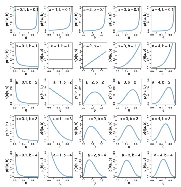
We use a generalization of the uniform distribution called the beta distribution. We choose it because it models values that are between 0 and 1. It is characterized by two shape parameters, usually labeled “a” and “b”, so it’s called a “Beta(a,b)” distribution and we would say p is distributed as a Beta(a,b) as follows:

For the uniform, we’ll pick a = 1 and b = 1. We would say that the prior is distributed as a Beta(1,1) random variable:

Next, what’s our likelihood? What’s our data model? We’re going to assume that each flip of the coin is independent of all the others and is identically distributed. Since the probability of getting heads is p, the probability of getting tails is 1-p. So the probability of getting 7 heads and 3 tails would be:

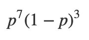
This “coin flip” distribution is called Bernoulli distribution.

How do we compute the posterior? I’m going to use a cheat here: If your prior is a Beta(a,b), and your likelihood is a Bernoulli with z successes out of N flips, then the posterior is also a beta, with the following distribution:

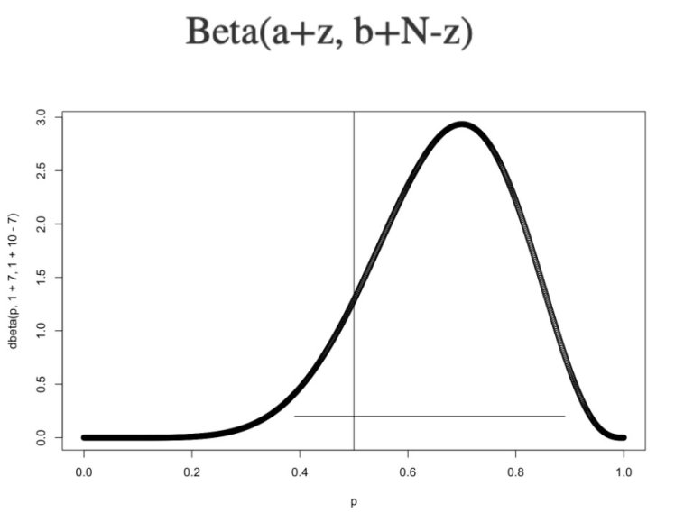
The plain horizontal line is the 95% highest density interval or HDI. It contains 95% of the probability. (There’s nothing special about 95%.) The fact that 0.5 is covered by the HDI means that it’s not inconceivable that this is a fair coin. With only 7 flips, it’s hard to be definitive. I would conclude that these coin flips are not significant evidence of a trick coin.

The HDI is a kind of credible interval. Interpreting a Bayesian credible interval is very intuitive; the proverbial “person on the street” probably thinks of probability this way. This ease of interpreting results is a big plus for Bayesian inference.

This went so quickly because of our “cheat”. The official name for the cheat is that beta and Bernoulli are conjugate pairs. When two distributions are conjugate pairs, the posterior is very easy to calculate. There are several conjugate pairs.

But what happens when you want to model something that doesn’t have conjugate pairs? Until the 1990s, you couldn’t. The distributions couldn’t be solved analytically.

Bayesian inference with MCMC and probabilistic programming

Without our coin flip example, we only have one variable to predict. If we had hundreds or thousands, we’d be out of luck. And that is a totally different problem from being unable to solve the problem analytically.

Markov Chain Monte Carlo (MCMC) changed all that and brought about a Bayesian revolution. MCMC is a fascinating and complicated topic, but it roughly works like this: instead of trying to solve a complicated distribution analytically, we draw samples from it by creating a special Markov chain that explores the distribution.

The most important part for research is that users no longer have to do this themselves. All you have to do is define your model and let the MCMC sampler do the job for you. Now we can solve our problem using a probabilistic programming language.

Here’s how to solve our coin-flip problem with probabilistic programming, namely the PyMC3 module in Python.

import arviz as az
import matplotlib.pyplot as plt
import numpy as np
import pymc3 as pm

observed_flips = np.array([7]) # 7 heads out of 10 flips

with pm.Model() as model:
    # prior
    p = pm.Beta("p", alpha=1, beta=1)
    # likelihood
    flips = pm.Binomial("flips", n=10, p=p, observed=observed_flips)
    # inference
    trace = pm.sample() # produces 1000 samples

idata = az.from_pymc3(trace) # make plot
az.plot_trace(idata);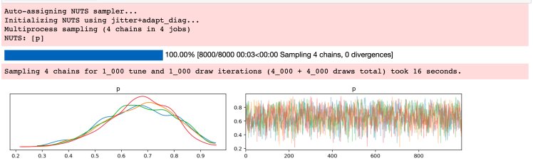

“NUTS” here is “No U-Turn Sampler”, the MCMC engine doing the inference. I have 4 cores on my local machine here, so it created 4 Markov chains, each with 1000 samples, each one getting a histogram in the left panel. Each of them looks like the analytic result from above. The right panel shows all four samples superimposed (the x-axis here is “sample number”). Looking at your samples this way can indicate the general health of your chains.

With PyMC3, we can also look at the posterior and HDI:

pm.plot_posterior(trace['p'], ref_val=0.5, bins=30, color='skyblue'

, hdi_prob=0.95)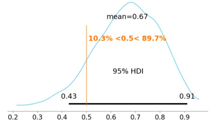

We get the same result as before, but with a lot more polish. We even get the percentage of probability that’s on either side of our reference line; maybe we would reject fairness if there were only 5% probability on the left side of the interval.

Even though we have an exact answer in this case, this procedure of specifying your model in a programming language and inferring what you need from the posterior distribution is exactly the same for more complicated models.

The BEST Test: do two samples have the same mean?

BEST, or “Bayesian Estimation Supersedes the t-Test”, was designed to be a robust alternative to null hypothesis testing (NHST). For our purposes, NHST may be good enough for what we need it for. But BEST will give us more information if we need it.

If you’re going to do probabilistic programming, there’s a nifty graphical shorthand to describing the models. For example, the model we just fit looks like this:

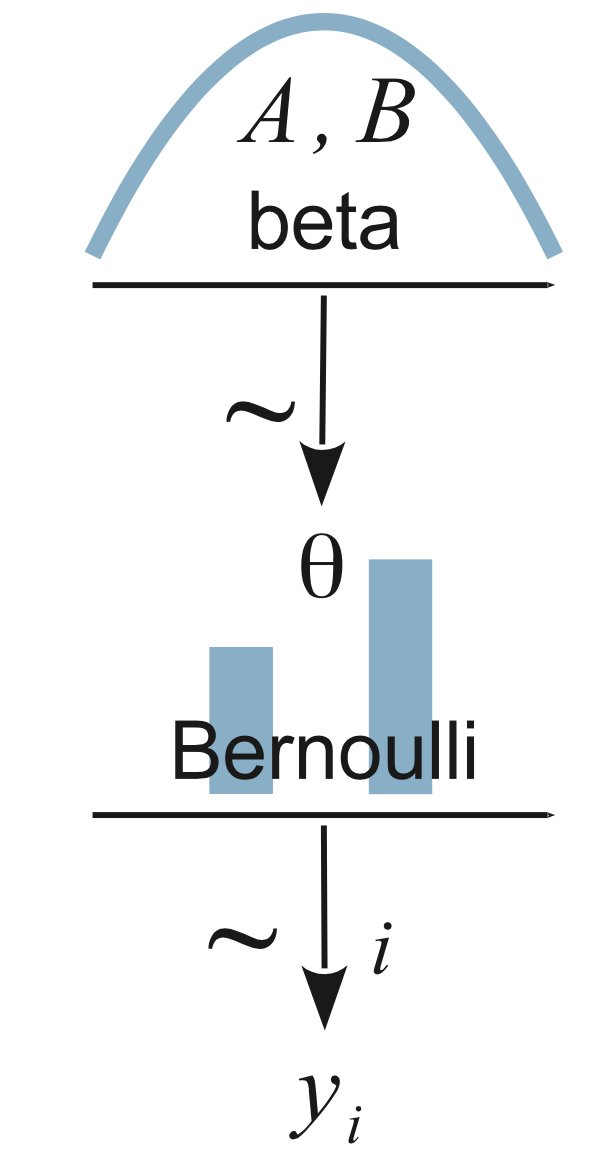
Read it from the bottom-up. The y are the observed pattern of heads and tails. We model that with a Bernoulli distribution, with theta being the probability of heads (p above). The prior for theta is a beta, as we said earlier.

Here’s the diagram for the BEST test:

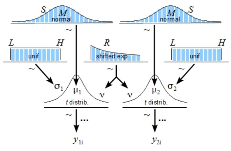
y1 and y2 are two data sets. Each of them is modeled with a t-distribution, which is like a normal distribution (mean mu, standard deviation sigma) with an extra parameter (nu, called “normality”) that controls how heavy the tails are. The t-distribution gets used in NHST as well. Every parameter in a Bayesian inference has to have a prior, shown as the blue distributions in the diagram.

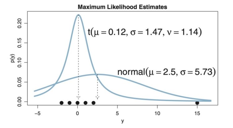
t-distributions are useful here because they are robust. They accommodate outliers without shifting the mean and variance:

One way if deciding if these two data set actually have two significantly different means is to find the posterior distribution of the difference of their means. Imagine giving some test patients a new smart drug, and giving others a placebo. Let’s say that for patients in both groups that we take a bio-measurement (say, diastolic blood pressure in mm/Hg). Can we conclude that the drug is having an effect? Can we conclude that the data could’ve arisen from the same underlying group? Can we conclude that the difference in means is consistent with zero?

When you implement this diagram for a made-up data set, you get:

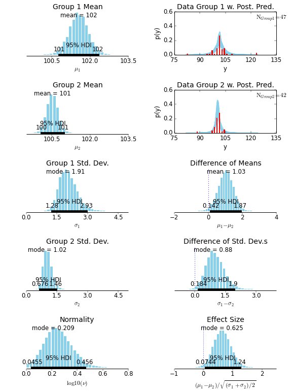
The data are the red histograms in the upper right. The money plot we care about is in the lower right, with a “Cohen’s d”-like measurement. We can see that, for this data set, the overlap with zero is very small, and we can consider these two data sets to be significantly different.

Bayesian inference is coherent and flexible, and is only limited by our imaginations! (That, and a good MCMC sampler. But otherwise: imagination!)